Implement Efficient File and Folder Structures – The Storage of Data

1. Decompress the ALL_SCENARIO_ELECTRODE_FREQUENCY_VALUE.zip file from Exercise 4.1 and upload it to the directory structure you created in Exercise 4.7, for example as follows. (Consider choosing year, month, and date folder names that align with your timeframe.)
   EMEA/brainjammer/in/2022/04/10/10
2. Create another directory that will contain the converted file, for example:
   EMEA/brainjammer/out/2022/04/10/11
3. Log in to the Azure portal at https://portal.azure.com ➢ navigate to the Azure Synapse Analytics workspace you created in Exercise 3.3 ➢ on the Overview blade, click the Open link in the Open Synapse Studio tile ➢ select the Develop hub ➢ click the + to the right of Develop ➢ select Notebook from the pop‐up menu ➢ ensure that your Spark pool is selected from the Attach To drop‐down list box ➢ and then execute the following code snippet, which is available on GitHub in the Chapter04/Ch04Ex11 directory:
   %%pyspark

df = spark.read.load(‘abfss://@.dfs.core.windows.net/in-path/file.csv’,

 format=’csv’, header=True)

df.write.mode(“overwrite”) \

 .parquet(‘abfss://*@*.dfs.core.windows.net/out-path/file.parquet’)

4. Check your ADLS container to confirm that the Parquet file was successfully written, and then execute the following code snippet:
   %%pyspark

df = spark.read.load(‘abfss://@.dfs.core.windows.net/out-path/file.parquet’,

 format=’parquet’, header=True)

print(df.count())

5. Create the following folder structure in your ADLS container. (Consider choosing year, month, and date folder names that align with your timeframe.)
   EMEA/brainjammer/cleansed-data/2022/04/10
6. Execute the following code snippet, which loads the Parquet file from the out path into a DataFrame and creates partitions for year and month:
   %%pyspark

from pyspark.sql.functions import year, month, col

df = spark.read \

.load(‘abfss://@.dfs.core.windows.net/out-path/file.parquet’,

format=’parquet’, header=True)

df_year_month_day = (df.withColumn(“year”, year(col(“SESSION_DATETIME”)))) \

.withColumn(“month”, month(col(“SESSION_DATETIME”)))

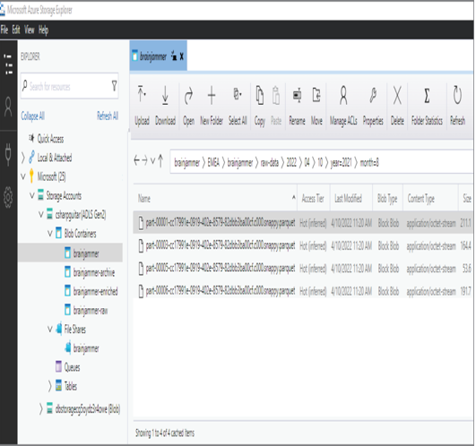
7. Execute the following code snippet, which writes the files into the partitioned directories. The output files should resemble Figure 4.34.
   %%pyspark

from pyspark.sql.functions import year, month, col

df_year_month_day.write \

.partitionBy(“year”, “month”).mode(“overwrite”) \

.parquet(‘abfss://@.dfs.core.windows.net/EMEA/brainjammer/cleansed-data/2022/04/10’)

FIGURE 4.34 An efficient file and folder structure

8. Query the data files on a specific partition as follows, replacing the * with your endpoint details:
   %%pyspark

df = spark.read \

.load(‘abfss://@.dfs.core.windows.net/path/year=2021/month=7’,

format=’parquet’, header=True)

print(df.count())

display(df.limit(10))

9. Consider committing your notebook to GitHub.

The folder from which the data files are retrieved and to which they are written are intuitive in the following ways. The original file is located within the file path that identifies the region, the ingestion direction, and a date. Looking at the following path, you can conclude the data is coming from EMEA and is brainjammer data sent/received on the date in the path:
EMEA/brainjammer/in/2022/04/10/10

The original data file format is ingested as CSV and converted to Parquet, which is a more efficient file format for querying. The converted data file is placed into an out directory, which signifies that some kind of ingestion operation was performed on it, and it is now ready for further transformation or optimization. One way to make querying more efficient is to partition the data file, like you did in steps 5 and 6 in the Exercise 4.12. You stored the partitioned files in a folder named cleansed‐data, which represents a phase of the data landing zone (DLZ). Recall this from Figure 3.8 in the previous chapter.
EMEA/brainjammer/cleansed-data/2022/04/10

In all three of the actions, there is a timeframe that is closely related to the location where the files are stored. Additionally, the data itself is also stored in folder structures based on dates like year and month. This storage structure makes the removal, i.e., pruning, of the data more efficient because it is easier to locate and determine if it is still relevant. If it is determined that the data is no longer relevant, especially the data in the in and out directories, then the data can be removed. Partitioning data results in the files being smaller, which makes removing portions of the file or the entire file itself less latent.